Did you know… About the “Mid Between 2 Points” OSnap?

It hasn’t been around forever, but this Object Snap is such a handy little tool you’ll wonder how you ever managed to live without it! The best news is that it’s available both in AutoCAD and IntelliCAD.

Whenever you’re prompted to “Specify a point:”, you can enter “M2P” at the Command: line or you can hold your shift key + right-mouse to display the pop up box and select “Mid Between 2 points” option. This allows you to snap to the MidPoint between two other points. The pop up box is shown below.

Mid Between 2 Points


Next you’ll be prompted to specify two new points for which you can use additional OSnap settings. The example below shows a new line that starts at the Midpoint between the ENDpoints of the two existing lines.Finding the MidPoint Between Two ENDpoints


Special Offer from Esri for Carlson IntelliCAD Users

Since the focus of my class and of the NC Surveyors Show as a whole is GIS, I thought it made sense to bump the information about the free copy of Esri software to the top…

Those currently using Carlson with IntelliCAD are eligible for a new “GIS Starter Kit” from ESRI. The Kit includes:

  • ArcGIS ArcView desktop software
  • A copy of the book A to Z GIS: An Illustrated Dictionary of Geographic Information Systems
  • A copy of GIS Tutorial: Workbook for ArcView 9, Third Edition
  • A 10% discount for the ESRI Survey & Engineering GIS Summit ($325 – standard registration price)

To take advantage of the offer, call 1-800-GIS-XPRT (1-800-447-9778) and request the Carlson-IntelliCAD GIS Starter Kit and please have your Carlson Serial Number available.

You can read more about ESRI’s commitment to survey and engineering services by visiting http://www.ESRI.com/engineering.


Did you know… About the Upright flag for linetypes?

I didn’t until this weekend.

While working on a new Picks and Clicks article for Professional Surveyor magazine I stumbled on something incredibly handy. This setting keeps text that’s inserted into a linetype in an Upright position rather than allowing it to be upside-down. 

Notice the polyline in the picture below. The top segment (drawn from left to right) has the text upright but the bottom segment (drawn from right to left) shows the text upside-down.


text is upside-down in linetype

The reason this happens is because of the definition of the “GAS_LINE” linetype in the acad.lin file.

The R=0.0 parameter formats the linetype text so that it aligns with the line segment. Therefore, whether text is upright or upside-down depends on the direction the line is drawn. However, if you simply change the R=0.0 to U=0.0, the polyline displays like this:


text is upright in the linetype

Notice the text is now upright in both segments. Using the U in the linetype definition sets the “Upright” flag. Setting it to 0.0 keeps it Upright relative to the line. I played around with it a bit and, unfortunately, it doesn’t seem to help much when rotating with DVIEW or UCS. But, when you’re working in world coordinates, this is a great tool.

To my knowledge this is a recently added enhancement to AutoCAD – but I thought it was cool enough to put up here!

My next column in Professional Surveyor will be… Surprise! Standardizing Linetypes! I’ll post a link here when it’s posted on their site. Follow this link to see if you are eligible for a free subscription to the print magazine: Subscribe to Professional Surveyor magazine.


Picks and Clicks: Field to Finish Follow Up

This article originally appeared in the December 2011 issue of Professional Surveyor magazine.

After we published “Understanding Field to Finish” in the September issue, I received more feedback and questions than I had for any other article to date. Although my plan for this month’s column had been “CAD Standards Part 2” (Part 1 is in the June issue), it makes more sense to answer some of the questions that were sent my way about Field to Finish first.

(I am using Carlson Survey for the examples in this article, but corresponding features and commands should be available as part of the Field to Finish feature of most other programs.)

The majority of readers’ questions revolve around how to code field descriptions and generate linework for multiple point codes. You use multiple point codes when you have a single field shot that defines more than one feature—for instance, a shot that locates both an edge of pavement and a sidewalk. However, before diving too quickly into multiple point codes, let’s make sure we have a good understanding of the different ways that you can use descriptions and linework codes to generate linework.


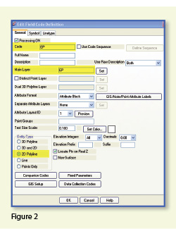
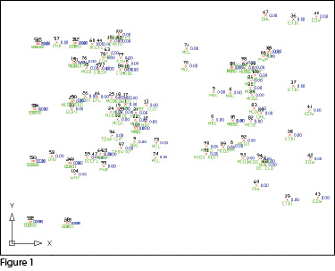
In Figure 1, the dotted lines represent the actual edges of pavement that exist in the field. Points 1-10 have a description “EP” designating them as Edge of Pavement.

When locating features that are generally symmetrical and that have two “sides,” such as a road, a sidewalk, or even a ditch having two tops of bank, we have a choice in how best to collect the points. Depending on field (and traffic) conditions, it may make more sense to take all the shots along one side of the road before crossing the road and taking all the shots along the opposite side.

The other way to collect shots is in what we call Zorro fashion: where we crisscross the street, taking shots on both sides, as we progress down the road. You can see that we used the Zorro style when taking shots in Figure 1. Point 1 is on the northwest side of the road, and shots 2 and 3 are on the southeast side. We then crossed back over to the northwest side to pick up 4 and 5, and so on.

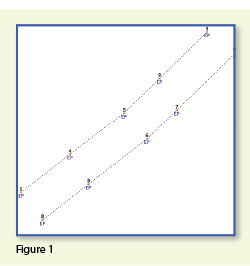
To draw the linework for the edges of pavement, you must create a field code for the EP description. You can see from Figure 2 that it requires only a couple of specific settings to indicate that this is a 2D polyline type of entity and on what layer the polyline is to be created.

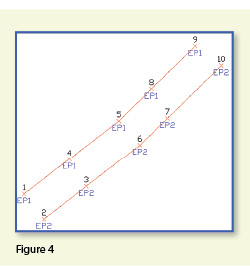
With the EP field code defined, using Field to Finish to draw points 1-10 generates the linework on layer “EP” (shown in red in Figure 3). Obviously this is not quite what we expected. I like to say that this is an example of the software doing exactly what we told it to do … rather than what we meant to tell it to do. So, we need to make a couple of adjustments.

The software understands only that it’s expected to connect all of the EP points with a 2D polyline. Carlson Survey allows you to choose whether the field code points are connected in “Sequential” order or “By Nearest Found.” The default setting is “Sequential,” which is why it connected the points the way it did. Unless we provide a little more information, there is no way for it to differentiate one edge of our pavement from another. If we make a minor change in the descriptions we use, we can have the program generate the linework correctly.

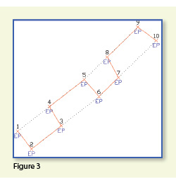
Rather than calling all edge of pavement points EP, we can use a number to modify the description so that we can tell the two polylines apart. We can use “EP1” for the northwest side and “EP2” for the southeast side. Now, when we redraw the points using Field to Finish, we end up with Figure 4, which is exactly what we wanted.

It is important to note that the field code does not change even though we’re now using EP1 and EP2 instead of EP. The field code is still “EP.”

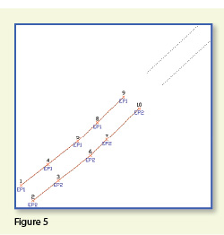
Let’s introduce just a little more complexity. Beyond points 1-10, we have an extension of this road with two additional edges of pavement that are shown as dotted lines in Figure 5. We do not want to continue the linework from points 9 and 10 but to start new polylines instead.

If we use descriptions EP1 and EP2 for the new edges of pavement, Field to Finish will assume we are continuing the other edges of pavement. So we must, again, have a way to differentiate the new edges of pavement from the ones drawn previously.

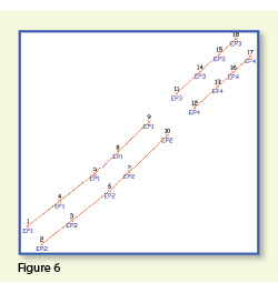
Using the same method as in the prior example, we can use descriptions “EP3” and “EP4” for the new edges of pavement. As you can see in Figure 6, this leaves us with the four separate polylines that we wanted.

The only drawback here is that the numbering of each distinct edge of pavement could get confusing on a large site. In this example, once they’ve been used, EP1 or EP2 can’t be used again without Field to Finish thinking all the EP1 points are part of the same polyline.

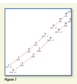
The good news is that it only requires another small coding difference to allow you to re-use EP1 or EP2 again. In Figure 7, we still use the EP1 and EP2 descriptions, but we use them in combination with special linework codes “+7” and “-7.” In Carlson lingo, “+7” is the default code to “Start a new polyline” and “-7” is the code to “End the polyline.” You can see that once we have descriptions “EP1 -7” and “EP2 -7” at points 9 and 10, we start new polylines by reusing EP1 and EP2 at points 11 and 12. As long as you’re diligent about using the “-7” special linework code to end the previously drawn polyline, you can reuse the descriptions.

Multiple Point Codes

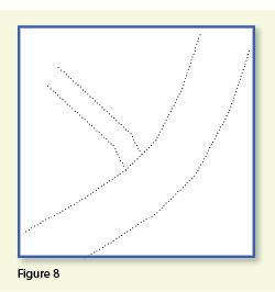
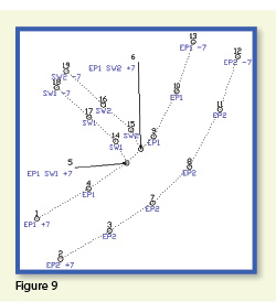
You use multiple point codes when you have two site features (such as the edge of pavement and a sidewalk) that intersect. As you can see in Figure 8 there are two points where a sidewalk meets the edge of pavement. In Figure 9, you can see the descriptions we used so we could have Field to Finish process points 5 and 6 as part of both the EP and SW linework entities.

Point 5’s description “EP1 SW1 +7” means that this shot is a vertex along the current EP1 polyline and also starts a new polyline named SW1 to define the edge of the sidewalk. Point 6’s description “EP1 SW2 +7” means that this shot is also a vertex along the current EP1 polyline and starts another new polyline named SW2 for the other side of the sidewalk.

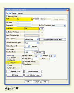
To have Carlson’s Field to Finish process these points as shown, we had to create only one additional field code: the “SW” code for sidewalk. We set the Entity Type to 2D Polyline and set the Main Layer to “SW” (Figure 10).

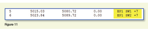
Now, let’s take a closer look at the descriptions for points 5 and 6 (Figure 11). In Carlson Survey, if you use a space between two descriptions, the program allows you to process them separately using the two corresponding field codes. The corresponding field codes used to process these descriptions are EP and SW so Carlson will process the same point twice, first using the EP field code and then again using the SW field code.

Because having a space in a point description is an indicator to Carlson that multiple field codes may need to be processed, it is a best practice to avoid using spaces in your descriptions. Using a description such as 24” RCP PIPE can create several problems, but the main one is that Carlson will think it is supposed to process three separate field codes: one for 24”, one for RCP and one for PIPE. A better description would be PIPE/24” RCP. In this example, a field code named PIPE would be processed. And, because a forward-slash (/) separates PIPE from 24” RCP, Carlson considers everything after the slash as a comment and will ignore it when processing Field to Finish.

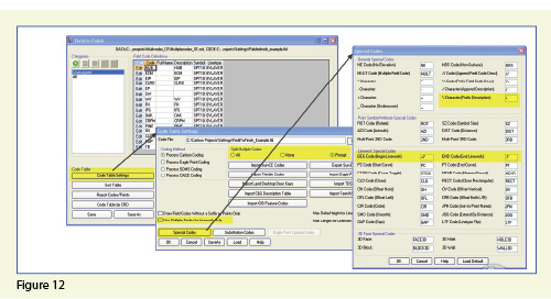
If you follow the maze of dialog boxes in Figure 12, there are several settings to take note of:

  • In the Code Table Settings dialog box, there are three possible settings for Split Multiple Codes.
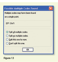
  • If you select “All,” any point description that contains a space will be processed as a multiple point code. If you select “None,” all spaces will be ignored when it comes to processing multiple point codes. If you select “Prompt,” you will be prompted with the dialog box from Figure 13 each time a space is encountered in a point description.
  • In the Code Table Settings dialog box, select the option to “Use Multiple Codes for Linework Only.” This causes Carlson Survey to create both the EP and SW linework on their respective layers but only one point (created on the layer specified by the first field code). If you do not select this option, the program will create two points with the same point number but with different descriptions. Each point will be inserted on the layer specified by its respective field code.

In the Special Codes dialog box, you can see the default settings and are able to customize the Special Codes used to process descriptions, points, and linework in Field to Finish.

With that, I hope I’ve been able to answer a few more of your Field to Finish questions. Please don’t hesitate to call or email as needed. I hope everyone has a fantastic holiday season, and I’ll see you back here in 2012!

This article originally appeared in the December 2011 issue of Professional Surveyor magazine.


Picks and Clicks: Understanding Field to Finish

This article originally appeared in the September 2011  issue of Professional Surveyor magazine.

Don’t be intimidated!

DEFINITIONSField to Finish—A general term used to describe the process of automatically drawing survey field data based on point descriptions and other field codes.Field Code (Description Key)—An alphanumeric code, corresponding to the point’s description, that defines how points are processed using Field to Finish. For points to be sorted onto a particular layer, be included in a point group, have a symbol inserted, or have linework that connects points be automatically generated, a Field Code having the point’s description must first be created.Field Code File (Description Key File)—A file that contains all of the Field Codes. 

Linework Codes—Codes entered before or after a point description that, when processed using Field to Finish, indicate where linework starts and ends or how to create additional, associated linework.

Somewhat like the seemingly Herculean task of developing CAD standards that I wrote about in the June issue, Field to Finish is one of those topics that almost everyone attending my workshops or training classes wants to learn more about. If they are not using Field to Finish, they think they should be—and, if they are already using it, they think they could be doing more or doing it better.

For those who are unfamiliar with it, Field to Finish is a general term used to describe the process of automatically drawing survey field data based on point descriptions and other field codes.


Depending on the survey software you use, Field to Finish may include some or all of these tasks:

  • insertion of survey points on to separate layers based on the point’s description,
  • sorting of points into point groups,
  • “tagging” of points, based on the point description, as “non-surface” points (this means that the points, even if selected, will be ignored when building a surface model),
  • insertion of a symbol onto a separate layer based on the point’s description or note,
  • rotation or scaling of a symbol based on the point’s description or note, and
  • drawing of 2D and/or 3D polylines connecting points based on the point’s description or note.

Although most survey programs can perform these or other tasks that fall under the Field-to-Finish header, to my knowledge, Carlson Survey is the only one to have commands or files that are actually named “Field to Finish.”


Land Desktop and AutoCAD Civil 3D use the term “Description Keys” for their feature that sorts points onto separate layers and inserts, rotates, and scales symbols. A separate feature called “Automatic Linework” or “Process Survey Linework” generates the polyline figures in these programs. For purposes of this article, Field to Finish refers to the generic term and, unless otherwise specified, applies to any survey program.

Benefits

For those who have never used Field to Finish, it can be summarized in one word: intimidating! But once you see what can be accomplished with a little extra coding, I believe you’ll be convinced it’s worth it. Because a picture is worth a thousand words, it’s easier to show you the benefits of Field to Finish.

The generic command for importing points (rather than Field to Finish) was used to import the points in Figure 1. In addition to overlapping attributes that make it hard to read, the points are all on the same layer, making connecting the dots even more time consuming and difficult.


However, if you use Field to Finish to import the points into the drawing, it looks like Figure 2. The points have been frozen in this view, but you can see the symbols and 2D and 3D linework that have been generated on their proper layers.


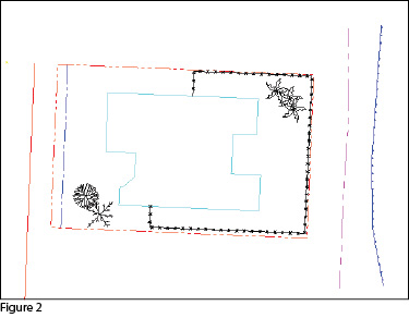
Granted, these examples demonstrate the power of Field to Finish when used to its fullest capacity, and it does require additional time and attention in the field to generate these results. In my training classes I encounter a lot of skepticism from folks who don’t believe the extra time in the field is worth it. While it may look cool, they say, it’s just easier to sort to layers, insert symbols, and connect the dots manually back in the office.

Bite-size Pieces

I respectfully disagree—and I believe that tackling significant changes in procedure is best accomplished with bite-size pieces rather than one big bite. Do you remember how you’re supposed to eat an elephant? One bite at a time, of course!

  • Nibble: Sort points onto separate layers and into point groups.
  • Snack: Tag points such as fire hydrants and inverts of manholes as “Non-Surface” points.
  • Bite: Specify symbols to be inserted on points where needed.
  • The whole enchilada—er—elephant: Also use special linework codes to connect points using lines or 2D polylines (for plan generation) and 3D polylines (for defining breaklines for surface models).
Point Description ConsistencyRegardless of the level of Field to Finish automation you strive for, the single biggest key to success with Field to Finish is consistency among the point descriptions. If you are attempting to implement Field to Finish for the first time and want to ensure buy-in from your field crews, allow them to help develop the list of descriptions. After all, they are the ones having to enter them in the field. If the folks in the field are not consistent with the descriptions they enter for each shot, Field to Finish is doomed to fail.For instance, in the office, it doesn’t matter whether the description for a fire hydrant is “FH,” “HYD,” or “FIRE HYDRANT.” Once the Field Code File has been created, it’s simply a matter of processing the Field to Finish routine. So, rather than someone in the office dictating what descriptions the field crew should use, ask the crew what description makes most sense to them and what they are confident they can remember and enter every single time.


Even though the “nibble” part seems simple enough, it still requires a considerable amount of thought and consideration. So, how do you start? First, determine what descriptions will be used for shots taken in the field. In order to use Field to Finish, you will need to create a field code for each description that may be processed now or in the future.


Start by going back to one or two of the largest point files you’ve worked on recently and sort it out based on the point descriptions in it. Use this list as a guide to determine what descriptions to keep and what to throw out and also to trigger your memory for other descriptions that may be used in the future.


Once you’ve completed your list of descriptions, each description must be defined as a Field Code (Description Key) in the software. It’s during this step that layers can be assigned for the points, symbols can be specified for insertion, point groups can be defined, and non-surface points can be tagged. Depending on the software you use, the dialog boxes and interface will be different, but the data and settings entered are generally the same.


For Carlson Software users, there is a routine in the “Draw Field to Finish” dialog box that automatically creates a Field Code Table (populated with Field Codes) from a Coordinate File. If you’re not using Carlson Survey, I recommend opening your point file in Microsoft Excel to sift through and sort the list of descriptions.


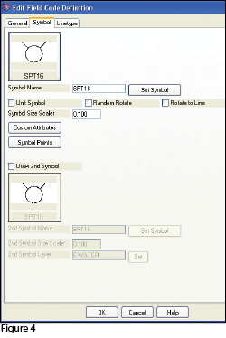
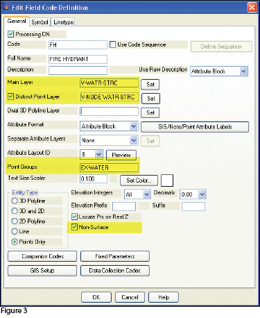
The Field Code that processes points with an FH description, as defined in Carlson Survey 2012, is shown in Figure 3. On the “General” tab of the dialog box, note the highlighted areas that show the layers, point group, and the checkbox to tag points as non-surface. Importing points with an FH description and using the “FH” Field Code definition results in the symbol named SPT16 being inserted on the layer V-WATR-STRC, the point being inserted on layer V-NODE-WATR-STRC, and the point included in a point group named EX-WATER.


The “Symbol” tab of the dialog box (Figure 4) is where you specify the symbol name and various other rotation, scale, and insertion settings.

Connecting All Your Points

As I stated previously, it’s a reasonable goal to get to the point where Field to Finish is used to sort points and/or symbols onto their proper layers and into point groups and to tag some points as non-surface to keep them from being included in a surface model. These are office-only tasks, because using Field to Finish to complete them does not require anything from the field crew other than consistency when entering point descriptions.However, the ultimate goal is having Field to Finish connect all of your points with 2D and/or 3D linework. Compared to the previous tasks, this requires more buy-in from the field crew because of the additional coding and noting.


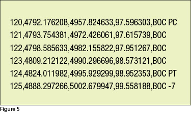
In Figure 5 you can see the linework coding that has been added to the “BOC” (Back of Curb) point descriptions in the sample of the point file. The “+7” linework code instructs the program to begin drawing linework, and the “-7” instructs it to stop drawing that piece of linework. The “PC” and “PT” identify the starting and ending points of a curve that fit all points in between the PC and PT.

The Field Code that processes points with a BOC description is shown in Figure 6. If you use the linework codes from the point file along with the BOC Field Code definition, it results in a 2D polyline on layer V-ROAD-CURB-BACK that starts at point 119 and goes to point 120. Then it goes into a curve that best fits between points 120 and 124 and ends with another tangent line from point 124 to point 125. A 3D polyline connecting the same points will also be drawn on layer 3D-EXISTING. In addition, the points will be inserted on layer V-NODE-CURB-BACK and included in a Point Group named EX-ROAD.


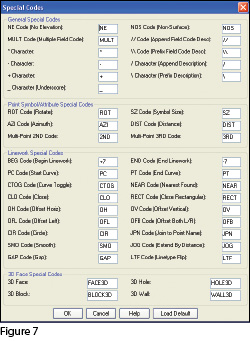
And this is just a sample of what can be done using Field to Finish. Depending on your software and data collector firmware, there are many other linework codes that can be used to automate the creation of linework based on your point descriptions and notes. In some cases there are specific linework codes that must be used, such as “B” for Begin linework (instead of the +7 used above) or “E” for End linework (instead of -7). Other programs, like Carlson, allow you to customize these codes. The “Special Codes” dialog box in Figure 7 shows the default linework codes used in Carlson Survey 2012.


I have one last piece of advice for those who are considering jumping into the world of Field to Finish for the first time. Cheat! Well, kinda. Every survey program with a Field to Finish feature has sample files that you can use as-is or modify to meet your needs. Rather than starting from scratch, it’s sometimes easier to work with one of those prepared files.


As always, I encourage you to send your feedback or contact me with questions at [email protected].

This article originally appeared in the September 2011 issue of Professional Surveyor magazine.


Picks and Clicks: The Key to Standardizing Annotation in CAD Files

This article originally appeared in the June 2011  issue of Professional Surveyor magazine.

Part 1

The issue of CAD standards has long been one of my pet projects when working with clients. It’s the universal problem, as folks from every office confess that CAD standardization is either “non-existent” or, at least, “could be better.”

In my experience, the single most-intimidating aspect to developing a CAD standard is deciding how to standardize annotation in order to accommodate the multiple scale factors used in a typical plan set. Other types of sheets surveyors and civil engineers may have to produce are:

  • a cover sheet (at 1:1 or no scale),
  • one or more project or phase site plan sheet (at 1:50, 1:100, 1:500, 1:1000, etc.),
  • plan and profile sheets (at 1:30, 1:50, etc.), and
  • detail sheets (at 1:1 or no scale).

It’s not an easy issue to resolve, and CAD programs seem to vary from bad to worse in their ability to manage multiple scales within a single CAD file.

Some of the information provided here is very basic, but in my experience even long-time CAD users struggle a bit with the “under-the-hood” details about annotation sizing. So, that being said, where should you start?

Determine the Plotted Size, Plotted Height, Plotted Distance … of Everything

The most important first step when developing a CAD standard for annotation is to determine the desired plotted size of annotation entities. And, when we discuss annotation, we must remember that this encompasses more than just text; it also means linetype patterns and dimension styles.

Here are several sample questions to ask when developing a CAD standard for annotation:

  • When plotted, what is the height (in inches) of the text displaying:

– the project title in the title block?

– the road name?

– contour labels?

– 
property line bearings and distances?

  • When plotted, how far off the property line (in inches) should the bearing and distance label be placed?
  • When plotted, what is the distance (in inches) between labels along a contour?
  • When plotted, what is the length (in inches) of the arrowheads at the end of dimension objects?
  • When plotted, what is the distance (in inches) that the extension line extends beyond the dimension line?
  • When plotted, what is the length (in inches) of the dashes and gaps in the linetype used to show existing contours?

Overwhelmed yet? Don’t be. Once you commit to the size or height of a few entities, the rest come fairly easily just because you know that you want one entity a little smaller or a little bigger than another.

The remainder of this column covers the issue of standardizing text sizes in your CAD files. Future columns will cover the other questions relating to linetypes and dimension styles in much more detail.

Standardizing Text Sizes and Placement

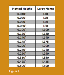
Although text height can be set to any desired value, the most commonly used height for plotted text in civil/survey drawings is 0.08”. There are several other standard text styles (corresponding to the height of the plotted text), known as “Leroy,” that have been adopted from the days of hand and technical lettering. Even though the “Leroy” text style usually has a Simplex font, the naming convention is widely accepted to describe text of a specific height regardless of its font.  For instance, L80 text refers to a Leroy style text that plots 0.08” high; L100 is Leroy with a plot height of 0.10”; and L200 is Leroy with a plot height of 0.20”. Other standard heights and style names are shown in figure 1.

L80, or text that plots 0.08” high, is generally used for basic text such as bearings and distances, contour labels, and notes. For more prominent text such as road names or parcel numbers an L150, or text plotting 0.15”, may be used.

You may be saying, “Yeah, that’s great and all, but when I enter text it asks me for the height of the text to be placed in the drawing, not its plotted height.” If you use the generic commands for placing text, that is true. However, most civil/survey programs have specialized commands for labeling that also take into account a horizontal scale that you specify independently for each drawing.

For instance, in Carlson Software or Civil 3D, you can specify program defaults so that bearing and distance labels always have a plotted height of 0.08”. Then, as each new drawing is started, you set its horizontal scale. For a drawing with a horizontal scale set to 1”=50’, the bearing and distance labels will be placed in the drawing at a height of 4.0’ (0.08 x 50 = 4.0). For a drawing with a horizontal scale set to 1”=100’, the bearing and distance labels will be placed in the drawing at a height of 8.0’ (0.08 x 100 = 8.0). The plotted height never changes.

Consider what a written standard for annotation would look like if we did not base the standard on the plotted size but on the actual drawing size of text…

  • In all 50-scale drawings, bearing and distance labels shall be placed in the drawing at 4.0’ high.
  • In all 100-scale drawings, bearing and distance labels shall be placed in the drawing 8.0’ high.
  • In all 50-scale drawings, all property corner labels shall be placed in the drawing 3.0’ high.
  • In all 100-scale drawings, all property corner labels shall be placed in the drawing 6.0’ high.
  • Unless otherwise specified, all other text in a 50-scale drawing shall be placed in the drawing 4.0’ high.
  • Unless otherwise specified, all other text in a 100-scale drawing shall be placed in the drawing 8.0’ high.

Now, with the understanding that all annotation sizes must be scaled by the horizontal scale, we can simply say:

  • All road names shall be L150.
  • All property corner labels shall be L60.
  • Unless otherwise specified, all other text shall be L80.

As you can see, because the text sizes refer to a plotted height, it makes the writing of CAD standards for annotation remarkably easier.

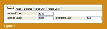
It is also important to note that, when placing text in a drawing, parameters other than text height can be adjusted to get the desired look. One of these 
parameters is the distance a label is placed above or below the line it labels.  Figure 2 shows a clip of the Annotate Defaults dialog box in Carlson Survey 2011.

The text height is specified using the “Text Size Scaler” value, and the distance that text is offset from the line it labels is specified by the “Text Offset Scaler.” Both of these values are “plotted” distances in inches. You can also see the horizontal scale setting for the drawing. Once plotted, text placed using these settings will be 0.08” high, and it will be positioned 0.04” off the line. A good rule of thumb is to set the offset value at one half the text height.

Another example of an annotation standard that can be associated with a plotted distance is how far apart to place elevation labels along a contour. Rather than specifying that contour labels are “300’ apart in a 50-scale drawing” or “600’ in a 100-scale drawing,” your standard should state that: On the plotted sheet, contour labels shall be shown at 6” intervals along each index contour.

I hope this information has provided a good kick-start toward your CAD standardization goals and helps get you thinking in plot sizes rather than drawing sizes. As noted above, future columns will focus on other supposed standardization nightmares such as dimension styles and will also touch on some specifics of the different CAD programs. Please don’t hesitate to contact me if you have questions. I hope your summer is off to a great start!

This article originally appeared in the June 2011 issue of Professional Surveyor magazine.


What is LandXML?

This article originally appeared in the April 2011  issue of Professional Surveyor magazine.

The ability to import and export LandXML data has been around for quite a while, but I still get a lot of curious looks when I mention it in my training classes. So, what is it, and why should you be using it?

What Is LandXML?

LandXML refers to a file format (.xml) containing data that has been generated from a civil engineering or land surveying software program.

If you’re hearing about it for the first time and want to learn more about the uses and acceptance of the LandXML initiative, visit www.landxml.org. According to their page LandXML.org in a Nutshell, “… LandXML.org is committed to providing a non-proprietary data standard (LandXML), driven by an industry consortium of partners.”

Simply put, the easiest way to convert, transfer, and archive data between Civil 3D, Carlson Software, Land Desktop, Eagle Point, TerraModel, and many other programs is to use the Import from LandXML and Export to LandXML functions available in these programs. Additionally, many machine control systems allow you to import LandXML files. I am most familiar with the Carlson and Autodesk families of civil/survey programs, so most examples in this article refer to them.

This may not be current by the time you read this article, but the list of members and participating organizations is at www.landxml.org/org.htm.

Why You Should Use It To Transfer Data

The two key words in the mission statement above are “non-proprietary.” Just as we have multiple proprietary drawing file formats such as .dwg (from Autodesk’s AutoCAD-based programs) and .dgn (from Bentley’s Microstation), the files that store survey and civil data such as points, surfaces, centerlines, and profiles are unique and proprietary to their manufacturer.

For instance, Civil 3D is the survey/civil product for Autodesk. Points and surfaces created in that program are stored inside the .dwg file. If you have Civil 3D and need to share a surface with a consultant or other team member who owns the same version of Civil 3D, you can just send them the .dwg file and they will have full access to the point and surface data. However, if you have Civil 3D and your consultant uses an earlier version of Civil 3D, Land Desktop, or Carlson Software or needs the surface data for machine control, it will not be as simple as just sharing the .dwg file.

Similarly, surfaces created in Carlson Software are saved in a .tin file and points are stored in a .crd (coordinate) file. Anyone using Carlson Software or SurvCE data collectors can load these files in their native format. But, Civil 3D or other survey/civil programs can’t access them directly.

As you probably already know, when you have to pass this data onto someone using a different program, it’s a nightmare! This is where LandXML is a lifesaver.

I like to explain that you use Land-XML files in the same way you used to rely on .dxf files. It’s mostly outdated now, but a .dxf file is a generic drawing file (DXF = Drawing Interchange File) that can be exported from and imported into various CAD programs. Back in the day, AutoCAD wasn’t able to read or import Microstation’s .dgn files and Microstation wasn’t able to read or import AutoCAD .dwg files, but both could export and read .dxf files. To get a Microstation file into AutoCAD, we had to export a .dxf file from Microstation and import it into AutoCAD and vice versa.

When you export your civil/survey data to an .xml file, it can be opened and read like a text file. Specifically, an .xml file is an .html file that is best viewed through a web browser such as Internet Explorer or Firefox. For instance, when a surface model (TIN) is exported to an .xml file, the X, Y, Z values of each point on the TIN are assigned a number, and then each “face” (triangle) of the TIN is defined by specifying the three corners (Figure 1).

Another benefit of using LandXML to transfer project data is that you can be selective in choosing what project data to include in your .xml file. For instance, in the course of a design project, you may create an existing ground surface, a proposed ground surface for phase one of your project, and a proposed ground surface for phase two. You may have a consultant who needs only your proposed ground surfaces. When you export the .xml file, you have the ability to select only those surfaces that you’d like to add to the file; it’s not necessary to export them all.

For Project Archiving

We’ve all become accustomed to saving archive copies of our drawing files for various purposes, but saving the corresponding project data such as points, point groups, surfaces, centerlines, and profiles is often overlooked. Retrieving the drawing file (.dwg or .dgn) may allow you to recover the linework that represents contours or a profile, but the underlying “surface” is lost unless the project data was also archived.

When archiving your projects at completion or even at submittal time, it is not enough to simply save a copy of the drawing file(s) for the project; you must also save a copy of the project data. At a minimum, the archive should contain the project data in its native format. In the case of Civil 3D, saving your project data in its native format means saving a copy of all .dwg files that store points, surfaces, or other data relating to your project. Saving this project data in its native format is sometimes the easiest method, but it can also create a problem with file storage because the files can become enormous.

This won’t be a surprise, but even if you archive your project data in its native format, I recommend that you consider additional archiving in .xml format. This is the case whether you need to save a progress, submittal, or final archive of your data. No one knows what kind of data files we’ll be using 10 or 20 years down the road, so saving your data in such a generic, text-based format such as .xml files allows for easier retrieval regardless of when you need it.

Note that, like archiving in native format, archiving to an .xml file can also produce very large files. I still believe using the .xml format is advantageous because of the generic nature of the data and having the ability to pick and choose the data you need to archive.

I hope you’ve gotten some clarification on this fantastic tool we’ve all had for years but many of us have not taken advantage of. If you have questions, please don’t hesitate to follow up.

This article originally appeared in the April 2011 issue of Professional Surveyor magazine.


Picks and Clicks: Conquer Problem Drawings

This article originally appeared in the February 2011  issue of Professional Surveyor magazine.

While working with IntelliCAD, AutoCAD, or any other AutoCAD-based programs, we’ve all 
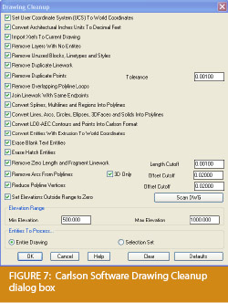
encountered the proverbial drawing from “you-know-where” that seems to drive us crazy from start to finish. Here I offer several tips to help you identify problems and conquer your problem drawings. I’ve listed these tips in the order I would apply them.

1 Purge your drawing.

The PURGE command removes any unused layers, linetypes, text styles, shapes (for linetypes and text), and many other items in the drawing.

When you run the purge command once, it will purge those items that are not currently in use and that have no other dependencies. For example, if a particular linetype definition depends on a particular shape, the purge command will delete the linetype definition only on the first pass.

Purging again will now delete the shape because the dependent linetype no longer resides in the drawing. Enabling the option to “Purge nested items” before purging will automatically execute the command repeatedly until all unused and dependent items are gone.

2 Purge remnants of registered applications that have accessed your drawing.

Typing “–PURGE” will execute the command line version of the purge command. This version includes a few options not available from the purge dialog box.

One of the extra options is “Regapps,” which is available only from the command line version of the command. You access it by typing “R” when prompted. This option removes “leftover” data from other programs (registered applications) that have been used to work on the drawing file.

3 Audit the drawing.

The AUDIT command looks for discrepancies between the objects displayed on the screen and the objects’ definitions in the drawing file database. The command then gives you the option of correcting the errors it has found. This command can be executed only while the drawing is open and active.

4 Recover the drawing and all reference files.

The RECOVER command is a more robust version of the audit command and can be used to open drawings that are so corrupt they cannot be opened otherwise.

Starting the recover command prompts you to browse to and select the problem drawing. If the problem drawing is already open and active, recover will prompt you to save changes before reopening the drawing and starting the recovery process.

For drawings that have attached XREFs (external references), use the RECOVERALL command to open and repair the selected drawing plus all dependent XREFs. Note that errors corrected by the audit are not saved back to the XREFs.

5 Block out the drawing contents to a new drawing.

If you suspect a drawing has become corrupt, you can WBLOCK the entire drawing out to another file. After starting the wblock command, set the “Source” option as “Entire Drawing” and provide the location and name for the newly created file.

Note that this command saves only Model Space entities to the new drawing. If needed, use AutoCAD Design Center to transfer layout tabs.

6 Insert the problem drawing as a block into a new drawing.

Using the same principle as above, you can use the INSERT command to bring the Model Space contents of a problem drawing into another drawing. Doing this will reduce or eliminate corruption in the problem drawing.

Make sure to use 0,0,0 as the insertion point and set the rotation angle and scale appropriately.

As with wblock, this command saves only Model Space entities to the new drawing. If needed, use AutoCAD Design Center to transfer Layout tabs.

7 Export drawings from vertical programs to AutoCAD.

Autodesk products such as Land Desktop or Civil 3D create program-specific, proprietary entities such as AEC Contours and AEC Point Objects. These proprietary objects can become corrupt or otherwise create problems when being accessed from standard AutoCAD or another program that doesn’t recognize the proprietary entities.

You can enter the -EXPORTTOAUTOCAD command at the command line to create a new drawing file that strips out the proprietary entities and leaves only standard AutoCAD entities. For instance, a Land Desktop or Civil 3D drawing containing AEC Contour entities will result in elevated polylines with text when exported to Autocad. And a Land Desktop or Civil 3D drawing containing AEC Point entities will result in a block with attributes when exported to AutoCAD.

Note that any AEC Objects will obviously lose their intelligence, but the new drawing can be opened in any version of Autocad.

8 Use DWG TrueView Convert to fix errors and bind XREFs.

DWG TrueView is a free program that you can download from Autodesk’s website. It is most valuable for its ability to convert drawings to earlier versions individually or in bulk. In the Conversion Setup dialog box, you can specify one or more options to clean drawings during the conversion process.

9 Use the Drawing Cleanup command in AutoCAD Map or Carlson Software.

Both AutoCAD Map and Carlson Software provide Drawing Cleanup commands that provide a variety of cleanup tools. In either version, you have the option of performing one or more cleanup tasks on the entire drawing or on only selected entities in the drawing.

Note: Use these commands with caution and apply cleanup options incrementally to avoid making unwanted changes. Also, I recommend making a backup copy of the active drawing before performing this command.

If you use AutoCAD Map, Land Desktop, or Civil 3D, you can access the Drawing Cleanup command from Map ➜ Tools. In Carlson Software, access it from the File menu.

10

I’ve come up with 9 tips that will help you clean up and, maybe, access drawings that have become corrupt. To round out the list and make it an even 10, I’d like to hear from readers to find out what your favorite drawing recovery and cleanup tools are. Please email me at [email protected] and I’ll report in a future column.

This article originally appeared in the February 2011 issue of Professional Surveyor magazine.


Picks and Clicks: Dynamic Blocks

This article originally appeared in the December 2010  issue of Professional Surveyor magazine.

Welcome to the first installment of this new column highlighting favorite AutoDesk, IntelliCAD, and Carlson Software features. My goal is to help you reduce your number of  “picks and clicks” while using these pieces of software so you can be more efficient, saving time and money.

Because many of us are hanging onto our current software versions for as long as possible these days, I will try to avoid reviewing features that were released in “last week’s” version and will instead write about commands and features that have been around for at least a few years.

First: A little about my background and experience. My first CAD class was with AutoCAD 9 and DCA software as part of my Surveying Technology coursework in college. After graduating, I worked for various consulting, engineering, and surveying companies where I used mostly the Autodesk family of products: AutoCAD, AutoCAD Map, Land Desktop, and Civil Design with brief detours into the MicroStation, GeoPak and Eagle Point worlds.

It was during this time that I started teaching basic CAD and civil/survey CAD classes at local community colleges. I then joined a local Autodesk and Carlson Software reseller to help start and build their training division. In 2004 I stepped out to begin working for myself as That CAD Girl. I offer Carlson Software sales; training and support for Autodesk, Carlson and IntelliCAD; and associated consulting services while specializing in CAD standards development and surface modeling training. My website is at www.thatcadgirl.com. And my surveying column is now here!


Water Valve

(Figure A)

One of my favorite, fairly new AutoCAD features is Dynamic Blocks, which was first introduced in AutoCAD 2006. A Dynamic Block is simply a standard block that has been enhanced with additional functionality. You may have seen examples of complex Dynamic Blocks that allow you to change the size (by stretching) or the orientation (by mirroring) only pieces of a block without having to EXPLODE it. But, you can also save many picks and clicks by giving your existing blocks a facelift with some simple Dynamic functionality. Let’s start with a standard symbol or block that most everyone will already have saved in a block library somewhere: a Water Valve.

To use the standard version of this block in a drawing, we usually have to:

  1. Use the INSERT command to bring the block into the drawing.
  2. Use a NEArest OSNAP to position the block on a line representing a waterline.
  3. Use the ROTATE command with the Reference option to align the block with the line.
  4. Whew!

Two minutes (or less) in the Block Editor will eliminate steps 2-4 (at right.)

  1. Insert the standard Water Valve block into your current drawing.
  2. Left-click to select the block.
  3. Right-click and open the Block Editor from the shortcut menu.
  4. On the “Parameters” tab of the Block Authoring Palette, select the tool to create an Alignment Parameter. [Figure B]
  5. The Command: line prompts you to, “Specify base point of alignment or [Name]:”. Use your 
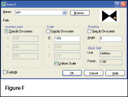
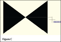
INTersection OSNAP to specify the insertion point for the block.
  6. Next, you are prompted to “Specify alignment direction or alignment type [Type] <Type>:”.  [Figure C]  Turn Ortho On and pick a point directly to the right of the insertion point.

  7. When finished, the block with its new Alignment icon will look like this in the Block Editor: [Figure D]
  8. 
Pick the Close Block Editor button at the top of the screen and then pick “Yes” when prompted to save the block definition.


Using the Dynamic Block

Once you are back in the main drawing screen, the original instance of the block will have been updated.

  1. Left-click the block to see the new Alignment icon.
  2. Left-click on the blue Alignment icon. This allows you to “pick up” the block and move it. [Figure E]
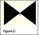
  3. Drag the block on top of a line in your drawing that represents a waterline. You will notice that, once your crosshairs are positioned over the line, the block automatically aligns itself to the line, and, in addition, the NEArest OSNAP is enabled allowing you to position and snap the block directly onto the line.
  4. Use the Insert command to draw additional copies of the block into the drawing. Notice that the thumbnail image of blocks with Dynamic parameters displays a lightning bolt icon so as to differentiate Dynamic Blocks from standard blocks. [Figure F]

Waterline Reducer

[Figure G]

Another often-used water-utility symbol that can benefit from the addition of Dynamic properties is the waterline Reducer. This symbol is used to indicate a change in the size of a waterline. In addition to an Alignment Parameter, this symbol needs a Flip Parameter that allows us to easily mirror it to change its direction. Unlike an Alignment Parameter, adding a Flip Parameter to a block also requires that you add a second Dynamic Block component called an Action. Giving a block “flip-ability” requires a few more steps, but is still rather easy.

  1. Repeat steps 1-7 as described for the Water Valve to insert the “Reducer” block into the drawing and add an Alignment Parameter to it. 
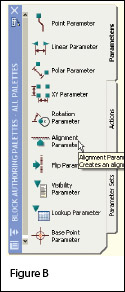
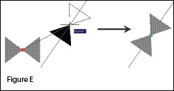
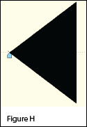
The Reducer with its Alignment icon is shown at left: [Figure H]
  2. Turn Ortho On.
  3. Pick the Flip Parameter icon on the Block Authoring Palette. [Figure I]
  4. The Command: line prompts you to “Specify base point of reflection line or [Name/Label/Description/Palette]:”. Use your ENDPoint OSNAP to specify the insertion point for the block (use the same point as for the Alignment Parameter).
  5. The Command: line next prompts you to “Specify endpoint of reflection line:”. With Ortho On, pick a point directly above the “Base Point” specified in the previous step. These two points define the “reflection line” for mirroring.
  6. You are then prompted to “Specify label location:”. Pick a point somewhere just above the Reducer symbol. The label reads, “Flip state”.
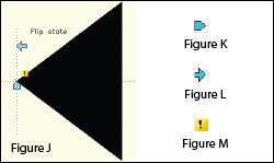
  7. Use the MOVE command, with Ortho On, to slide the Flip icon above the block.
  8. The Reducer [Figure J] with its Alignment  [Figure K] and Flip icons  [Figure L]  are shown at right. A Warning icon [Figure M] is also displayed indicating a missing Action component.
  9. On the “Actions” tab of the Block Authoring Palette, select the tool to create a Flip Action. [Figure N]
  10. The Command: line prompts you to “Select Parameter:”. Select any part of the Flip Parameter including the label, the Flip icon, or the Warning icon.
  11. Next, you are prompted to “Specify selection set for action. Select Objects:”. Select the Flip icon and all entities that make up the block/symbol.
  12. You are then prompted to “Specify action location:”. Pick a point somewhere near the “Flip state” label. The label has a lightning bolt icon and reads, “Flip”.
  13. Pick the Close Block Editor button at the top of the screen and then pick “Yes” when prompted to save the block definition.

Using the Dynamic Block

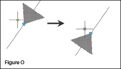
As before, once you are back in the main drawing screen, the original instance of the block will have been updated.

  1. Left-click the block to seea the new Alignment and Flip icons.
  2. Left-click on the blue Alignment icon to move it onto a line representing a waterline.
  3. Left-click on the blue Flip icon to mirror the block along the line.
  4. Use the Insert command to draw additional copies of the block into the drawing. [Figure O]

Note that the steps change the block definition in the current drawing only. The WBLOCK command must be used to save the block out as an external Drawing (.dwg) file.

This article originally appeared in the December 2010 issue of Professional Surveyor magazine.